


This article describes how mission scenarios created using gaming software can be used as a graphical concept of operations (CONOPS) and optimized to ensure the highest probability of mission success.
Traditional optimization methods have not been designed for mission-level problems, where highly uncertain environmental and operational parameters influence mission success, and clear objectives beyond success or failure are not well-defined. This unique class of problems requires new optimization processes. The case study in this article showcases a surveillance mission-level optimization problem with a graphical CONOPS and applies an efficient design space sampling strategy, surrogate modeling, and a value-driven multi-objective formulation to efficiently find an optimal solution. This new approach offers a method for diverse stakeholders to understand, communicate, and optimize system designs for complex and uncertain mission scenarios.
Two of the major ways that engineers use modeling and simulation are to support design decision-making and to provide realistic visual representations of scenarios. When dealing with complex systems, such as aircraft, these activities fall under the umbrella of model-based systems engineering (MBSE), where relevant domain models are connected to form a comprehensive model of the system lifecycle (Ramos, Ferreira, & Barceló, 2012). The overarching goals of MBSE are to enable systems engineering and design through a unified, coherent model, reduce the cost and time devoted to building and testing physical prototypes, and facilitate greater communications among stakeholders. However, there is still a marked disconnect between the subject matter experts who develop domain models and the higher-level decision-makers who perform trade-off analyses and set system requirements and objectives. This article proposes a new mission-level optimization approach to MBSE that integrates design optimization and trade-off analysis tools with a graphical concept of operations (CONOPS) to provide design solutions with the highest probability of mission success. By focusing on mission-level success, rather than system-level performance, and by using gaming technology to provide more realistic visual representations of system scenarios, this new approach brings these stakeholders closer together to support stronger and more mission-focused systems engineering and design.
Mission-Level Modeling through a Graphical CONOPS
Communicating design trade-off options to decision-makers and other stakeholders in an easily understood manner is important for delivering the best system possible. The concept of operations (CONOPS) document is a common method for systems engineers to present a proposed system design to these stakeholders. However, CONOPS documents can span hundreds of pages of dense text and tables, which limits their value for busy groups of decision-makers. One relatively new approach is to create a graphical CONOPS, where the information contained in a traditional CONOPS document is presented using gaming software that provides a visual simulation of the mission scenario. Presenting system characteristics this way can be a powerful method to simplify the decision-making process (Korfiatis, Cloutier, & Zigh, 2012). A graphical CONOPS is similar to using modeling and simulation to support wargames; however, the scope of the graphical CONOPS is generally more focused than that of a wargame. In a graphical CONOPS, the decisions that influence mission success are made before the simulation starts, and it therefore does not require the strategic layers seen in wargames.
While the stakeholders interact with the gaming software, “under the hood” is a collection of engineering models that control the physics of what is being shown on screen. The stakeholders have a dashboard from which they are able to set mission parameters, including how many actors are involved as well as important design inputs for the systems involved. One key characteristic of mission-level modeling is the need to characterize and represent sources of operational, tactical, and environmental uncertainty.
The example case in this article uses a graphical CONOPS mission simulation built in the Unity game engine. In this simulation, a blue “friendly” unmanned aerial systems (UAS) is searching for a target in a suburban environment, while a red “enemy” UAS maneuvers itself to block the path of the blue UAS. The blue UAS has a limited battery life, which is set by the design inputs and puts an upper bound on the amount of time it can search. If the blue UAS finds the target, the mission is considered a success. However, if the blue UAS crashes due to depleted batteries, the mission is a failure. Figure 1 shows a snapshot of the simulation in progress.
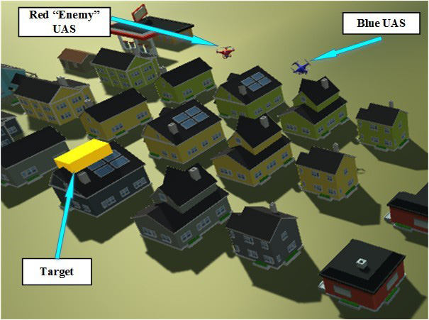
Figure 1: Snapshot of UAS/Counter-UAS Graphical CONOPS
The UAS flight trajectories are determined by a simple dynamics model. For the blue UAS, the destination it is traveling toward is randomly set every few seconds. The red UAS continuously attempts to collide with the blue UAS and knock it off its planned trajectory, while also occluding its camera view. The acceleration toward the destination for each UAS is determined by the distance to the target, where a larger distance requires greater acceleration. Specifically, the rotors apply a force related to a spring constant multiplied by the distance to destination, and this accelerating force is counteracted by a drag force. Collision forces and dynamics are handled by the collision software internal to the Unity software.
While the simulation is running, the blue UAS is constantly traveling around the suburban scene while the red UAS tries to block it. If the blue UAS comes within a threshold distance of the target while maintaining a line of sight to it, then the mission is successful.
This simulation has many inputs that can affect mission success or failure. Each UAS is defined by nine design variables that govern its geometry, power, and acceleration characteristics. Table 1 shows these simulation inputs, along with the upper and lower bounds programmed in the model. Several of these design variables are loosely bounded, and they are allowed to vary by more than an order of magnitude. However, even when the design variables are held to constant values, individual runs of the simulation have highly stochastic outputs. One set of simulations with constant inputs found a range in the time that the blue UAS took to find the target from a low of 1 second to a high of 25 minutes.
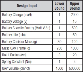
Table 1: Design Variables and Domains
The high number of input variables and level of output uncertainty raises a number of unique challenges for optimization. One of these challenges, for this and any scenario with high dimensionality and uncertainty, is that traditional optimization approaches would require many thousands of simulations in order to capture the likelihood of mission success across the design space. Running this many simulations would require a significant amount of time as well as extensive computing resources. Another challenge is that there are currently only two outputs that can be used as optimization objectives: The most important output is a binary parameter representing mission success or failure, and the secondary objective is a continuous parameter representing the time to find the target.
Complex System Optimization
A broad range of research has examined challenges related to the optimization of complex systems. Much of this is in the domain of multidisciplinary design optimization (MDO), which includes architectural techniques to manage different disciplinary or subsystem models, as well as algorithms and response surface techniques for optimizing simulation models. MDO techniques enable designers to ensure that subsystem interaction behavior is adequately modeled and that optimization is performed in an accurate and efficient manner (Martins & Lambe, 2013).
When the objective or constraint functions involve simulations, such as a computational fluid dynamics (CFD) model or a graphical CONOPS, a number of approaches are available to facilitate optimization. These methods can be broken down into four categories: random search and metaheuristics, ranking and selection, direct gradient methods, and surrogate model methods (Barton & Meckesheimer, 2006). Often, this choice can be difficult when the simulations include “black boxes,” where the underlying functions are unknown and only inputs and outputs can be used for analysis.
Another theme that is common to complex system design problems is the presence of uncertainty, which can be in the variables, parameters, or models themselves. While robust design optimization (RDO) and reliability-based design optimization (RBDO) (Paiva & Crawford, 2010) have been successfully used to optimize designs in situations where the uncertainty is low, such as in component tolerances, their applicability to scenarios with very high levels of uncertainty is limited. Both methods assume that the problems have well-defined constraints and well-known levels of uncertainty that can be analytically modeled. However, when optimizing for mission success, where many sources of extreme epistemic and aleatory uncertainty are present, alternative optimization approaches are needed.
What is Mission-Level Optimization?
Mission-level optimization has not been clearly and consistently defined in the literature. In this case, we refer to the optimal design of a system to successfully perform a job that takes place under highly varying external conditions. Crucially, the complexity of the mission scenario can bring about many different outcomes, and the most meaningful way to describe these outcomes is either success or failure. There are likely “intermediate” outputs, often referred to as key performance indicators (KPIs) when discussing system-level optimization, which may or may not be correlated to mission success but on their own do not account for environmental or operational factors.
Previous work that discusses mission-level optimization has largely focused on autonomous robot design and aerospace vehicles. Mission-level optimization of autonomous robots seeks the highest possible success/failure ratio when performing tasks such as maneuvering over an obstacle (Tesch, Schneider, & Choset, 2013) or grasping an object (Boularias, Bagnell, & Stentz, 2014). As in the current study, the objective is a binary success or failure output; however, their design variables relate to the robots’ behavior rather than the hardware design, and they do not account for high levels of operational or environmental uncertainty. The studies on mission-level optimization of aerospace vehicles typically refer to the tasks their systems perform as missions, using continuous objective functions that can leverage the optimization methods of more general problems (Bérend, Bertrand, & Jolly, 2007; Goulos et al., 2013; Yang, Luo, & Zhang, 2013). The key differences between the previous uses of the term and our definition are the emphases on the binary success/failure output and the presence of high levels of operational and environmental uncertainty.
Optimizing the Mission-Level Gaming Simulation
In order to simplify analysis, a “headless” version of the graphical CONOPS simulation was developed, in order to suppress the graphical user interface (GUI) and allow automated and accelerated simulation through command line arguments. This was then wrapped in the Phoenix Integration ModelCenterTM MDO software package to perform a diverse set of simulations using a “design of experiments” (DOE) (Myers, Montgomery, Anderson-Cook, 2016), evaluate the results, and perform optimization.
Due to the high stochasticity of the results even when the design variables are held constant, the mission-level objective is to minimize the probability of crash and failure, P(crash), over multiple runs of the simulation. Each set of inputs evaluated was run 20 times in order to characterize the different designs along this objective. In order to efficiently explore the design space, a DOE-based approach was leveraged using a definitive screening design (DSD) (Jones & Nachtsheim, 2011) with JMP 13 Pro Statistical Discovery SoftwareTM. Screening designs are useful for early design phases to quickly identify major trends in how the design variables affect the outputs. The DSD assesses each input at three levels, providing the ability to identify and potentially model curvature in the outputs when compared to a two-level screening design, which can only model linear effects. The DSD required 26 design variants, and with each replicate repeated 20 times, a total of 520 simulations were executed, shown in Table 2. Of the 26 unique design variants evaluated, 18 of them had a 100 percent mission success rate. The UAS designs that experienced failures show a wide range of success rates, with design variant number 24 having zero successful runs.

Table 2: Simulation Sample Inputs and Outputs, including Definitive Screening Design (DSD) and Optimal Solution
While mission success is the optimization objective in this case, the time to find the target is another important output that can be used to determine the best designs. By minimizing the mean time to find the target, µttf, the mission success rate will also, generally, increase. However, this can be complicated by the way that the model accounts for failed runs. For example, many designs with weak batteries actually have a low µttf, because the battery life will put an upper limit on the amount of time the UAS takes to find the target regardless of mission success. This means that while these designs have more failures, their successful runs will be completed very quickly; examples include designs 16 and 24 in Table 2. To address this issue, a bi-objective optimization problem can be formulated to minimize both P(crash) and µttf, which results in a Pareto-optimal set giving decision-makers information about the tradeoffs among the different objectives.
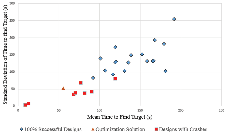
Figure2: Bi-Objective Plot of All Design of Experiments Runs with Optimal Solution
Analyzing the data from the simulation experiment using JMP Pro 13TM and ModelCenterTM, a sensitivity analysis was performed using only the successful runs to identify and rank model inputs by how much they influence the outputs. The analysis found that, for instance, the battery canister mass had very little effect on any of the outputs and could reasonably be ignored when creating surrogate models for the three objectives. On the contrary, the objectives are highly sensitive to the level of battery charge, which is used in the surrogate models.
For P(crash), a binary logistic regression model, a form of generalized linear models (McCullagh & Nelder, 1989), was trained. Firth penalized likelihood (Firth, 1993) was employed to account for the sparsity of design runs resulting in mixed results (both successes and failures). The surrogates for µttf and sttf were analyzed using loglinear variance regression models, which capture relationships between the input and output in both the mean and variance effects (Carroll & Ruppert, 1988). These models are then used to create a utility function to find the best design inputs depending on how much stakeholders weigh the three objectives against one another. The weights used for this analysis are 5 for P(crash), 3 for µttf, and 1 for sttf.
An optimal solution that maximizes this utility was found with a predicted P(crash) of less than 2 percent, µttf of 69.1 seconds, and sttf of 51.7 seconds. This design, seen at the bottom of Table 2, was then simulated 20 times in order to fully capture its behavior, resulting in an evaluated P(crash) of zero, a µttf of 55.4 seconds, and a sttf of 52.6 seconds. These results both fit the prediction very well and represent a significant upgrade over the other design points with a 100 percent observed success rate, even by using this relatively straightforward and efficient optimization technique. The upgrade in system desirability can be seen in Fig. 2, where the optimization solution is clearly better than any of the other solutions that did not experience crashes in their 20 simulated missions.
Conclusions
Mission-level optimization offers a new approach to designing systems in which the objective is to succeed at particular tasks under highly stochastic operational and environmental conditions. One way to do this that can engage multiple stakeholders is to link graphical CONOPS simulations with design optimization tools. The graphical CONOPS was originally developed to provide decision-makers with a realistic visualization of the system while also showing mission-level outcomes, supporting the vision of MBSE. Design optimization has long been used at the system level to maximize key performance indicators, which generally contribute to mission success but are not always synonymous with these higher-level outcomes. Combining these methods results in an improved approach to design for mission success.
The use case in this article demonstrates how mission-level optimization can be done for a relatively simple surveillance mission, where the optimization challenges are the high levels of uncertainty in environmental and operational parameters and the large number of design variables. Using statistical sampling, modeling, and optimization methods, an optimal system design was identified that had a simulated 100 percent mission success and better KPIs than any of the successful designs from the original sample, showing that mission-level optimization can be efficiently and effectively done with relatively small numbers of simulation executions, even in the presence of extreme variation.
As the systems engineering community advances its MBSE capabilities in linking multi-domain models into comprehensive representations of system behavior, the ability to optimize for success under highly stochastic mission scenarios will become increasingly valuable. Combining graphical CONOPS and state-of the-art statistical and optimization techniques can help bridge the communications and modeling gaps between strategic decision-makers and domain-modeling subject matter experts, while supporting the identification of optimal system designs for mission success.
References
- Barton, R. R., & Meckesheimer, M. (2006). Chapter 18 Metamodel-Based Simulation Optimization. Handbooks in Operations Research and Management Science, 13(C), 535–574. https://doi.org/10.1016/S0927-0507(06)13018-2
- Bérend, N., Bertrand, S., & Jolly, C. (2007). Optimization method for mission analysis of aeroassisted orbital transfer vehicles. Aerospace Science and Technology, 11(5), 432–441. https://doi.org/10.1016/j.ast.2007.01.007
- Boularias, A., Bagnell, J. A., & Stentz, A. (2014). Efficient Optimization for Autonomous Robotic Manipulation of Natural Objects. AAAI Conference on Artificial Intelligence, 2520–2526.
- Carroll, R. J., Ruppert, D., Stefanski, L. A., & Crainiceanu, C. M. (2006). Measurement error in nonlinear models: a modern perspective. Chapman and Hall/CRC.
- Firth, D. (1993). Biometrika Trust Bias Reduction of Maximum Likelihood Estimates Author ( s ): David Firth Published by : Oxford University Press on behalf of Biometrika Trust Stable URL : http://www.jstor.org/stable/2336755 REFERENCES Linked references are available on J. Biometrica Trust, 80(1), 27–38.
- Goulos, I., Hempert, F., Sethi, V., Pachidis, V., d’Ippolito, R., & d’Auria, M. (2013). Rotorcraft Engine Cycle Optimization at Mission Level. Journal of Engineering for Gas Turbines and Power, 135(9), 091202. https://doi.org/10.1115/1.4024870
- Jones, B. (2010). mODa 9 – Advances in Model-Oriented Design and Analysis, (October 2010), 0–15. https://doi.org/10.1007/978-3-7908-2410-0
- Korfiatis, P., Cloutier, R., & Zigh, T. (2012). Graphical CONOPS Development to Enhance Model- Based Systems Engineering. Development, (June), 18–20. https://doi.org/10.1073/pnas.0709132105
- Martins, J. R. R. A., & Lambe, A. B. (2013). Multidisciplinary Design Optimization: A Survey of Architectures. AIAA Journal, 51(9), 2049–2075. https://doi.org/10.2514/1.J051895
- Paiva, R. M., & Crawford, C. (2010). A Robust and Reliability Based Design Optimization Framework for Wing Design. Aerospace, 52(April), 2919–2919. https://doi.org/10.2514/1.J052161
- Ramos, A. L., Ferreira, J. V., & Barceló, J. (2012). Model-based systems engineering: An emerging approach for modern systems. IEEE Transactions on Systems, Man and Cybernetics Part C: Applications and Reviews, 42(1), 101–111. https://doi.org/10.1109/TSMCC.2011.2106495
- Tesch, M., Schneider, J., & Choset, H. (2013). Expensive function optimization with stochastic binary outcomes. 30th International Conference on Machine Learning, ICML 2013, n PART 3, 2320–2328. Retrieved from https://www.engineeringvillage.com/share/document.url?mid=cpx_52c24f28145700c9863M55a110178163125&database=cpx
- Yang, Z., Luo, Y. Z., & Zhang, J. (2013). Two-level optimization approach for Mars orbital long-duration, large non-coplanar rendezvous phasing maneuvers. Advances in Space Research, 52(5), 883–894. https://doi.org/10.1016/j.asr.2013.05.013